informationsbearbeitung

In the following posts we will explain, how to appy the findings about networks, to analyze the structure of multidimensional cubes.

We investigate the multidimensional cubes in orthogonal, Euklidean spaces, that means:

• the coordinate axes are orthogonal
• in Euklidean spaces of any dimension, the theorem of Pythagoras is valid

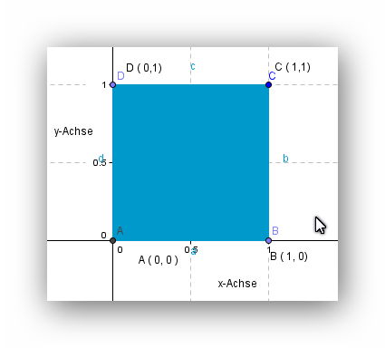
We start with a square in the  2-dim  Euclidean space and then go on to higher dimensions.

We use following conventions:

• the horizontal coordinate-axis is labelled as the x-axis
• the vertical coordinate – axis is labelled the y-axis
• both axis are orthogonal
• the length of each side, is 1  m

From that it follows:

1. dimension of Euclidean space = 2
2. area of square = 1 m^2
3. main diagonal  is AC   =  1.414  = BC

Now we imagine, that we are living in a two-dimensional world and that therefore we have no idea, how a cube in 3 dimensions will look like.

How can we find it out, by using only mathematical reasoning ?

At first we see, that we have to use 2 coordinate axes in 2 Dimensions and therefore  a 3. coordianate axis is needed, if we make calculations in 3-dimensional space.

Because  in 2 dimensional space we label each point with 2 figures, like P (  x,y ), we now have to label a point in 3 dimension as P ( x,y,z )

Because we cannot draw and construct a 3 dimensional cube, because we are living in a two-dimensional world, we can use only algebraic methods, because we also cannot visualize a cube in 3 dimensional space.

• We know, that the x, y and z axis must be orthogonal, because  now, we have a 3 dimensional Euclidean space.
• in 2  dimensions, we have a square with 4 corners. But how many corners will a 3 dimensional cube  have ? Because we cannot visualize a 3 dimensional cube, we don’t know it.

Therefore we have to check in detail, how we labelled the corner points of the square.

(0,0), (0,1), (1,0), (1,1)

Apparently, each coordinate of a point can have only the values 0 or 1 and all possible combinations of them  are used. Therefore we get 4 corner points.

We can go on one step further now, because the use of   o and 1 reminds us of the binary number system, like:

Now we can apply an elegant method, how to use number-labels for the corner points in a consistent way, which we can use also for multi dimensional cubes.

We transfer the binary numbers into decimal numbers

00  →  0

01   → 1

10  → 2

11   → 3

And we can use now these number labels, which will be much better for all calculations in multidimensional cubes:

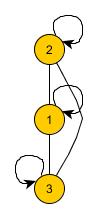
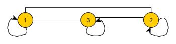
A   → 0,      B   → 2,     C  → 3,       D   →1

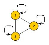
To get a bit familiar with this kind of labelling, we calculate the distances  L   between these points.

L01 = 1     L02 = 1   L03=1.414    L12 = 1.414   L13 = 1  L23 = 1

We get the lengths of  the 4 edges and the 2 diagonals.

The main diagonal goes from point 0 to point  3

L03 and L12 are calculated, using the Theorem of Pyhthagoras in othogonal triangles.

Now we repeat all steps, but for a cube in 3 dimensional space.

• because we have one additional  coordinate axis, we have to use 3 positions for the  binary numbers, to define each corner
• each binary number we transfer again into a decimal number

We remark following features:

• if the 3. coordinate is 0, then we get the projection of the 3 dimensional cube onto the 2 dimensional plane. That means, that the points 0, 1, 2,3  are the corner points of the square
• if the 3. coordinate is 1, then 4 new corners show up.
• in total we get 8 corners, which is  just  2^3

We could now calculate again all distances between these points  and would find:

• All edges have the length 1 m
• all diagonals in square faces have the length 1.414 m
• but we also get 4  new diagonals, which have the length 1.73 m

When we check, how we calculate these diagonals, we see, that the 3. dimension is included  in the Theorem of Pythagoras and that the lengths of these space diagonals is just the square root of the dimension of the cube.

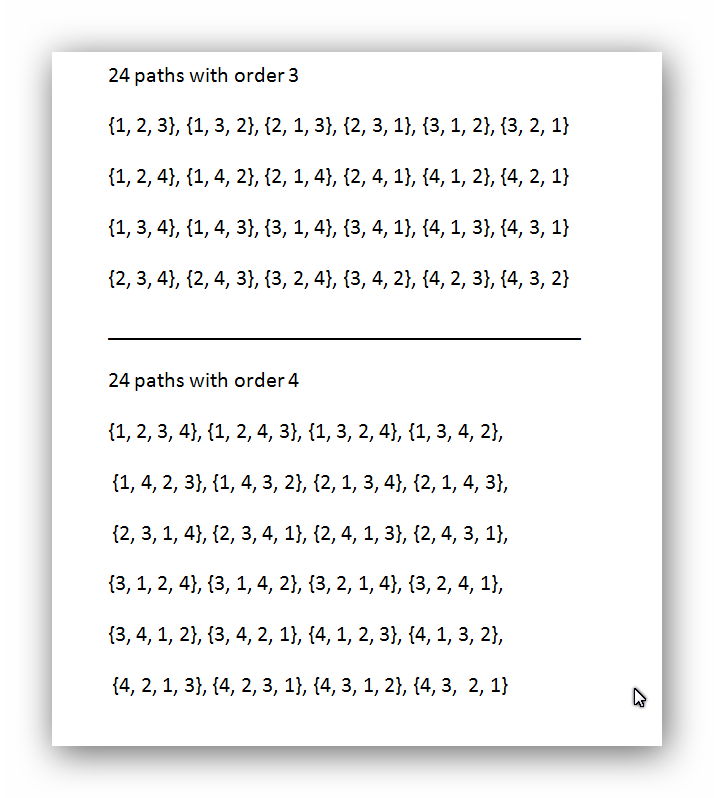
Now we could calculate the lengths  of all paths, whichever we like.

As an example we only calculate the length  the path 01234567

L 07 = 1+1.414+1+1.73+1+1.414+1 = 8,56 m

• Does there exist shorter paths, which use another sequence  of points, to come from point  0 to point 7, but which include  also each point only once ?

To summarize, what we found out :

• each corner point  of  a  cube in  an  n-dimensional Euclidean space, is defined by a binary number with n positions
• each corner can be labelled by using the decimal number, which is tranferred from the binary number representation of the corner coordinates
• the lengths of the edges are always 1 m and are  independent from the dimension of the space.
  • The same is valid for the areas of the faces of the cube; each is 1 m^2
• The volume is also always 1, but the unit for the volume is dependent on the dimension, like
  • area of square = 1 m^2
  • volume of 3 dimensional cube =  1 m^3
  • volume of 4 dimensional cube  = 1 m^4
  • volume  of n-dimensional cube = 1 m^n
• the lengths of the diagonals are also dependent on the dimension of the space

To understand better the structure of such cubes, we must find answers to several questions, like for instance:

• How many square faces do multidimensional cubes have ?

We know, that in 2 dimensions there is just 1 square face and in 3 dimensions there are 6 square faces. But these informations are not yet enough, to find any pattern, which correlates the number of square faces with the dimensions  of the cubes.

Because we cannot visualize cubes of higher dimensions than 3, we have to use again an algebraic approach.

We ask ourselves following:

• what characterizes a square face ?

Answer:

• each square face has 4 corners
• the distance beween neighbour corners is 1
• the diagonals have the lengths 1.414

But that does not yet help us, to answer the question, because there is still one problem:

• how do we know, that 4 corners are neighbour corners and are in the same plane ?

Definition:  a plane in a multidimensional Euclidean space is defined by 3 different points on it.

One straigthforware  method, to investigate, if all 4 corner points are on the same plane is, to calculate the equation for the plane, which is defined by  3  corner points and then check, if also the 4. corner points is on this plane.

Because that needs quite some calculations, I  postpone it a bit, hoping, that my  brain works a bit during sleep and finds a clever solution for it, which could save us a lot of work.

At least I have the feeling, that there must exist a much simpler method.